The following discussion on Facebook, Cathodic Protection Network public group is the motivation to publish a report on this subject.
Readers comments are in red and my responses and comments are in black.

If you want to join in please email me at roger.alexander3@ntlworld.com by copying and pasting this email address into your own email sender software.



Dear All.
I have a technical question.
does have the internal fluid conductivity effect on external cathodic protection of pipe or tank?
It seems that they are two independent phenomenas but the field survey and results means that conductivity of internal fluid affect on external polarization (corrosion potential and slope of Tafel curve). but i dont know the mechanism of this effect.
Do you know it?

Comment from another reader

Internal fluid conductivity will not effect on external cp system. only temperature can effect

My response: Sorry, I disagree.

PIPELINE-CORROSION-CONTROL.COM,Dynamic Project

PL. Explain. What is a role of Internal fluid? There is no role

My response
I have explained, briefly, in a few answers here but in order to really understand you should read my website. You will see that I have photographed and recorded all of my studies and am sharing them so that my time in existence will not have been wasted.

It is good that you are challenging and now you need to do what I have done and use your multimeter to prove what you think is true.

http://pipeline-corrosion-control.com/

Research
You must understand basic science to know that electrical energy passes from a higher potential to a lower potential, dependent on the conductivity of the available paths.
You can use Kirchhoff's Laws and Ohms law and use a spread sheet to calculate all of this.

Picture 1

You can also model this physically in a laboratory and gather real data in field work to fit in with real science and not the bullshit that is presently advocated.

2

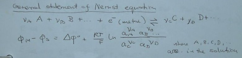
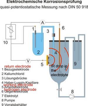
The Tafel curve and other formulae and equations are very nice in a classroom but you cannot actually MEASURE a potential, you can only measure a potential difference and that is a voltage.

Picture 3

Please read DIN 50918

Picture 4

Dear Alexander
So thanks for your kindly reply.
You are right, but Kirchoff's law at the node is valid when there is a potential difference (voltage) as a driving force. While in external cathodic protection, this difference in potential is between the structure and the anode that lies outside it. Therefore, the current leakage into the internal electrolyte has no driving force.

This is why I invented the Alexander Cell.

Picture 5


Please read the front page of my website as a start to understanding the real science. Then try it all out for real with your own meters and believe what the meters tell you.

http://pipeline-corrosion-control.com/

Kirchoff's law at the node is valid when there is a potential difference (voltage) as a driving force. While in external cathodic protection, this difference in potential is between the structure and the anode that lies outside it. Therefore, the current leakage into the internal electrolyte has no driving force.

My response: It is necessary to draw a simple circuit diagram to understand that I am correct.

Picture 6

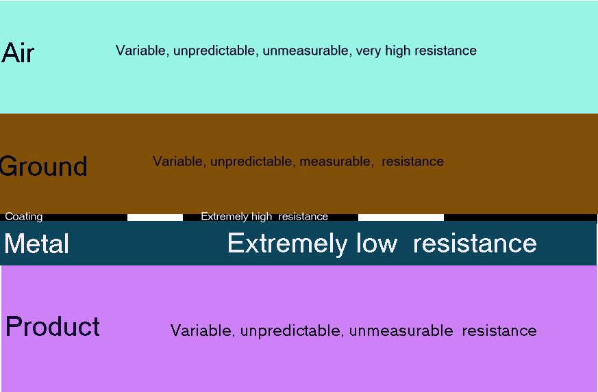
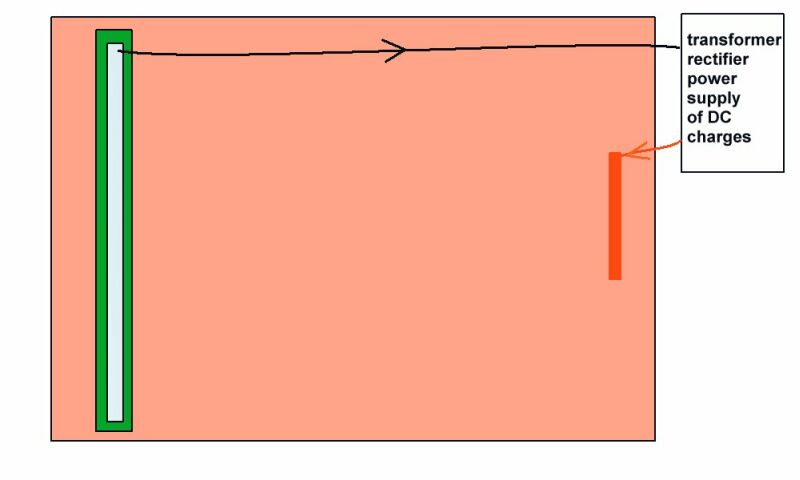
Let assume that the coating is totally resistant to electricity, but there are two coating faults.


Picture 7

Try not to complicate things by referring to electrons and ions as we cannot measure these.
Think in terms of electrical energy as that is what our meters and oscilloscopes measure in volts.
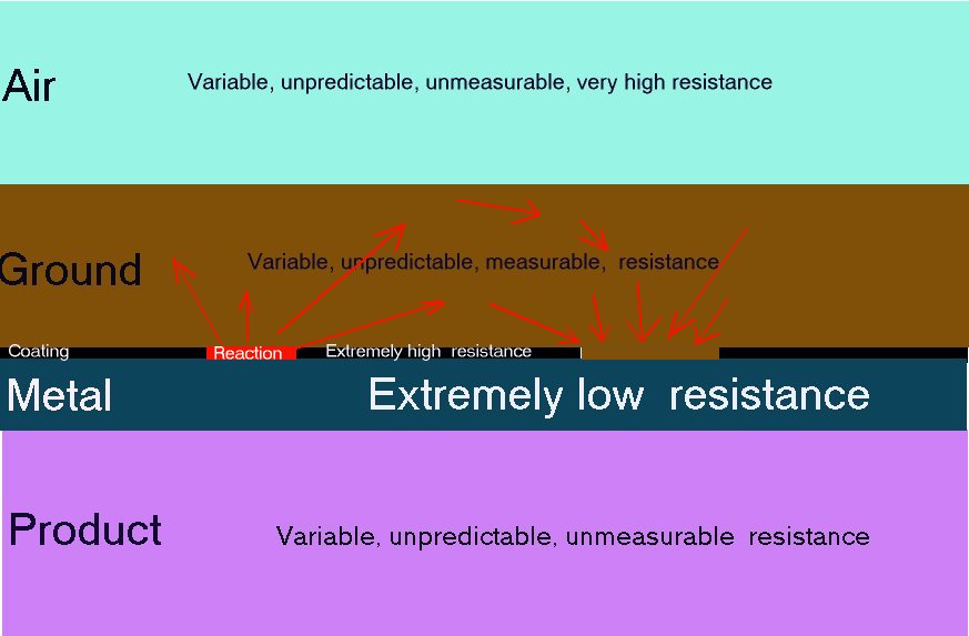
The corrosion reaction releases charges from the metal into the electrolyte as shown by the red arrows in this drawing.

Picture 8

Everything in the universe has an electrical potential that is trying to equalise with all the other electrical potentials and does this through the paths of least resistance.
Kirchhoff explained this.

Picture 9

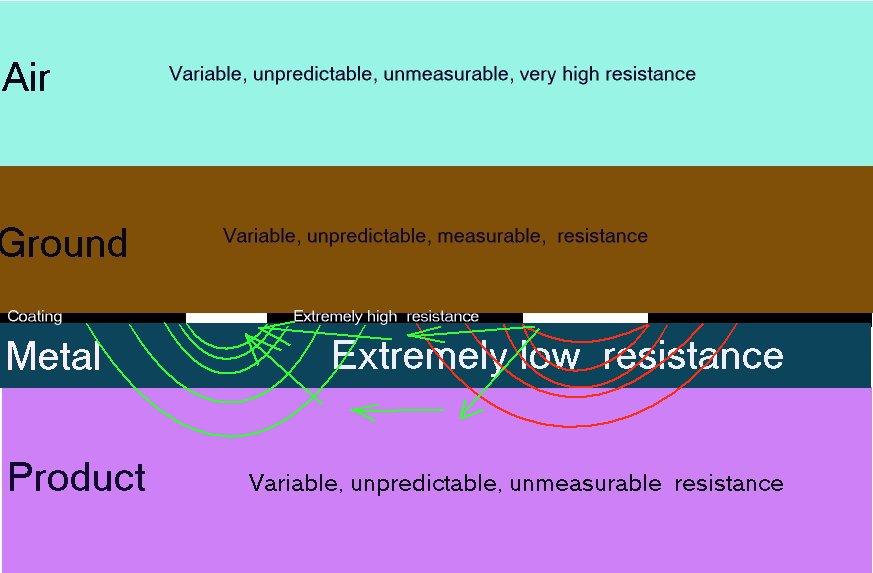
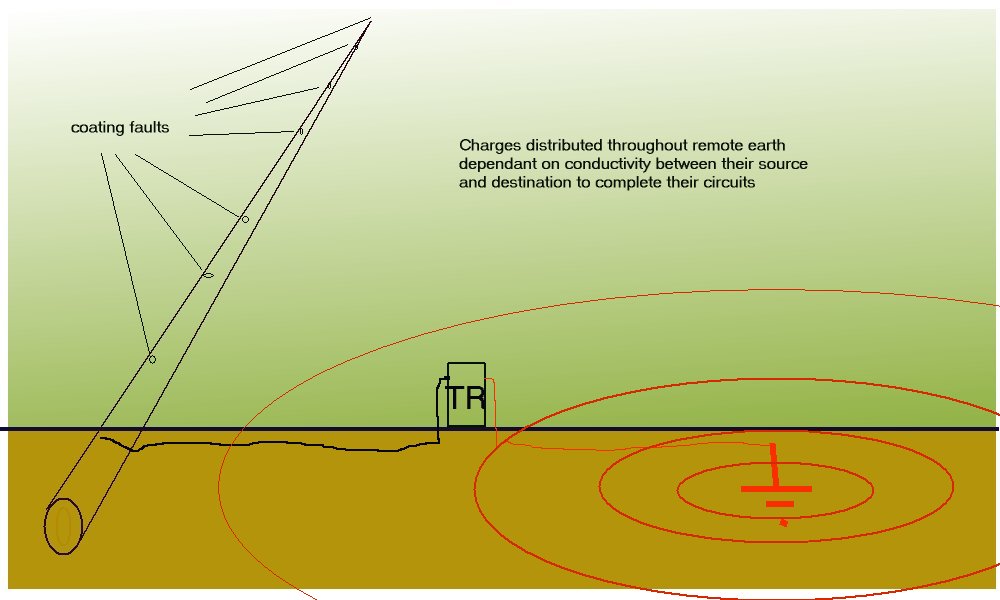
We are trying to stop the corrosion reaction between the subject metal and the electrolyte on the outside of the pipe or tank and for this purpose we 'pump' charges into the ground at the cathodic protection anode. These charges equalise out with remote earth and we drain charges from the subject metal at a drain point.
This is the cathodic protection impressed current circuit that reaches equilibrium. When we make a voltage measurement between any two nodes the meter assigns zero potential to the black (common input pole)

Picture 10

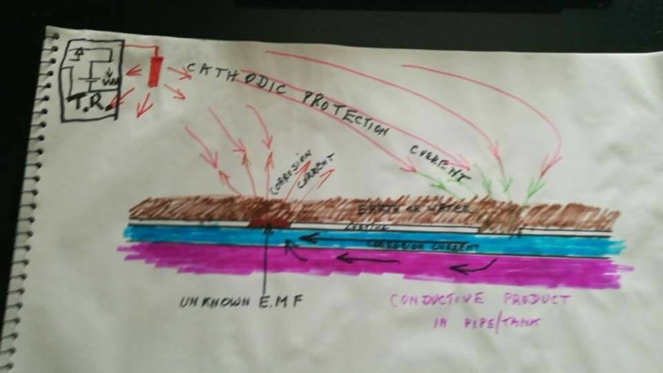
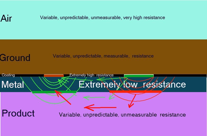
Let us assume that there are only two coating faults and that one is the anode and the other the cathode of this corrosion cell that we are trying to stop.


Picture 11

The metal of the pipe or tank has little resistance and it is impossible to measure this in field work but the corrosion current completes it's circuit through the metal.
However, if the product in the pipe or tank is conductive a portion of the charges will pass through this according to Kirchhoffs law of resistances in parallel.
I have repeated this drawing for your convenience as it is important to this discussion.

Repeat Picture 9

When we apply cathodic protection the extra charges will take the line of least resistance from the external anode to complete its own circuit. If there are external sacrificial anodes they will each have their own corrosion circuits.


Picture 12

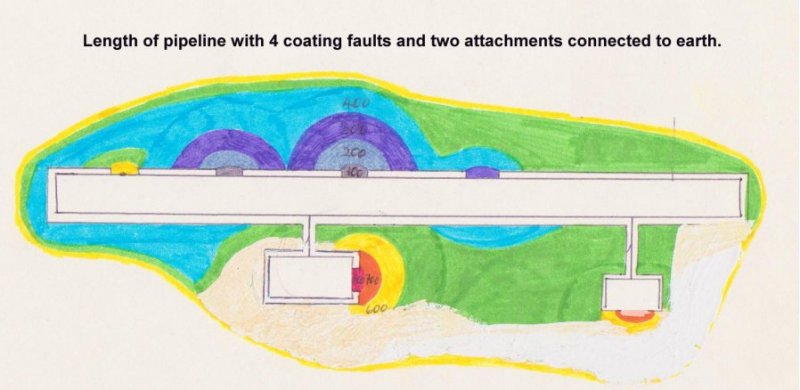
Using CPN techniques we can identify and quantify the effect of these on the corrosion equilibrium of the whole system.

http://pipeline-corrosion-control.com/

I know it and I know the mechanism of electrochemical corrosion and cathodic protection thermodynamically and kinetically. But I discuss about two different circuits (Internal and external circuits). The electrons can leakage into internal electrolyte if there is one positive pole but there is not positive pole in internal electrolyte because the anode is located outside. I am reading your front page about half cell now. It is very interesting and scientific. Let me to ask the probable questions about this.
Have a good time.

My response: Universal energy does not know any rules but it's own and I am lucky that I could not understand the rules that I was taught in school and by NACE and ICorr.... and the rest of the pseudo scientists, so I started rationalising from the very basics.

Although the metal of the pipeline or tank is extremely conductive it does no follow that it is all of one potential but that there are eddies of charges that go in and out of the metal according to the 'electrical pressure' at any given location in relation to the 'electrical pressure' in the electrolyte. This applies to the inside of the pipe as well as the outside.

Picture 13

Dear Alexander. I am so happy to know you. I try to learn more from you.

This next series of simple diagrams that explain the method of determining cathodic disbondment tests required by the coating industry written by Prof. Les Woolf for the British Standards Institute, who wrote me personally to confirm a paper I presented to the Institute of Corrosion Science and Technology in London in the 1980's.

Picture 14

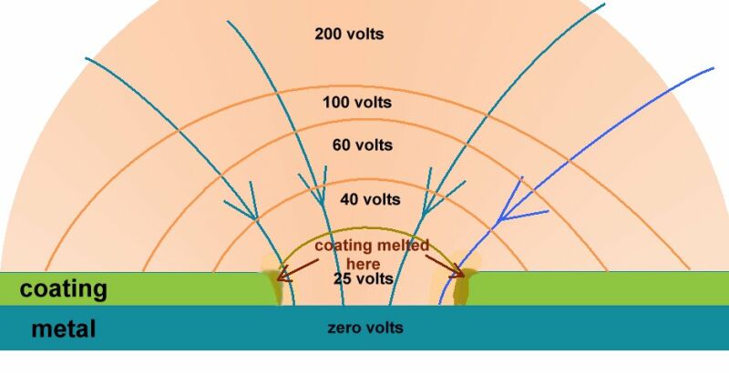
Prof. Woolf complained that his specifications were either misunderstood or deliberately ignored by industry and the testing authorities including Dr David Scantleberry of the Iniversity of Manchester Institute of Technology. In Picture 14 above you can see the specifications of Prof. Woolf's test and in Picture 15 below I have shaded the area to show the potential gradient in the electrolyte in the test tank that makes the exact distance of 10 mm vital.

Picture15

I visited Umist and saw the experimental set up and confirmed that it was incorrect and wrote to Dr Scantlebury who had failed to make a written report of my visit. He replied that I should get a book on electrochemistry and ignored my serious scientific questions.

Picture 16

In these next two pictures I have shown the potential gradient with the shells of resistance marked with typical values that can be measured by moving the silver/silver-chloride electrode.

Picture 17

Picture 18 shows the test if there is no coating fault. The charges spread evenly throughout the tank and no current flows.

Picture 18

This picture shows the current flowing from the whole of the tank into the coating fault to complete the circuit. I have also shown bubbles of hydrogen that have come from the crystaline structure of the metal thus causing resistance to the current and embrittlement if the current is too great. I have seen and measured this in casings of oil wells.

Picture 19

This shows the 'shells of resistance' as described by Dr Prinz in one of his papers that was given to me by Jim Gosden who was at that time Chairman of the Committee for BSI 1021

Picture 20

Note on this discussion:-
The metal of the pipeline or tank is very conductive and the inside of this metal is the same electrical potential as the outside. If the content of the pipe or tank is conductive it will be subject to Kirchhoffs laws of resistances in parallel and the charges will pass in inverse proportion to the value of each resistance in Ohms. This is how the shells of resistance are formed and can be measured in many of my experiments. Do not forget that all this is in 3D.

---

Experiment

In order to test these theories we must be able to gather data that shows that there are charges flowing inside the pipe as a result of energy passing from outside of the pipe. We must use instruments that are used in field work so that our observations can be compared to field data.

Picture 20

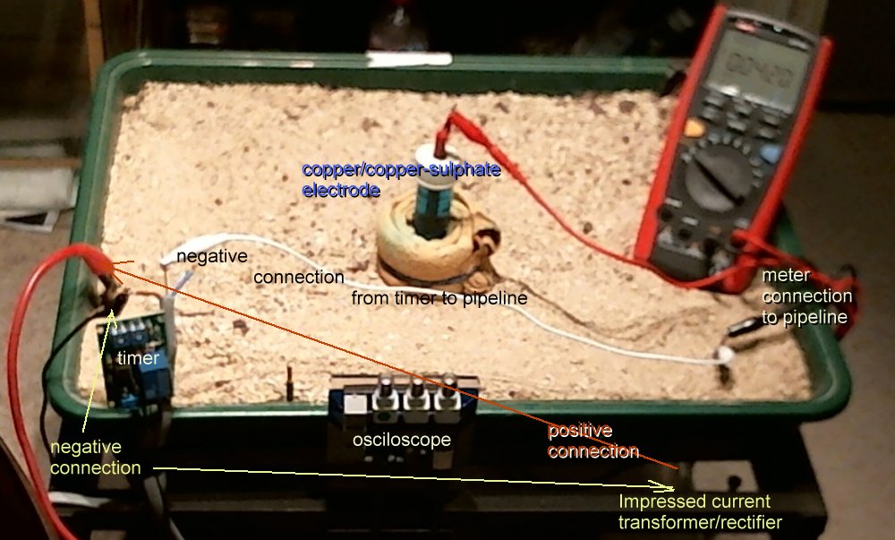
I am using two metal trays so that I can connect the positive output of the TR to each of these and replicate remote earth in that the charges will pass into the damp sand from all directions. Look at the picture and you can see

Picture 21

For those that do not understand the meaning of'remote earth' it is often refered to by electricians as 'ground'. When electrical charges are pumped into the ground they spread out in all directions according to the laws of electricity codified by Kirchhoff and others and follow the paths of least resistance to complete their circuit to their source. 'Remote earth' is where there are an infinite number of resistances in parallel making an infinitely low resistance. I have simulated this by charging both metal trays as 'anodes' in this experiment and the charges will return to the TR from all directions. They will meet resistance in the coating of the pipes but not at the coating faults. We can prove this by mapping a potential profile.

Picture 21

As a control I have set up a black, coated, steel pipe with two coating faults that I will later cause to be anode and cathode. This will create charges that pass through the electrolyte (damp sand and cloth) and return to complete the corrosion cell circuit through the pipe metal from cathode to anode as shown in Picture 8 above.

Picture 22

I will be using small copper/copper-sulphate electrodes to make all voltage measurements so that these values will match results in the field.

Picture 23

I am setting up a second steel pipe with a sharpened pencil plugged in each end as a method to measure the charges passing through the salt water. I have connected these to copper stubs in order that croc clips can make good connections to the meter.

Picture 24

I have set up a plastic tube of a similar length in a similar way so that I can measure the resistance of the salt water alone.

Picture 26

---

Resistance measurements

The first measurements will be the resistance measurements through each of the pipes and salt solutions. These measuremnets are made in the multimeter by sending a 9 volt charge from the positive pole and measuring the volts drop to the negative pole.


Picture 27

In Picture 27 you can see that the circuit resistance is 15.99 k Oms.

Picture 28

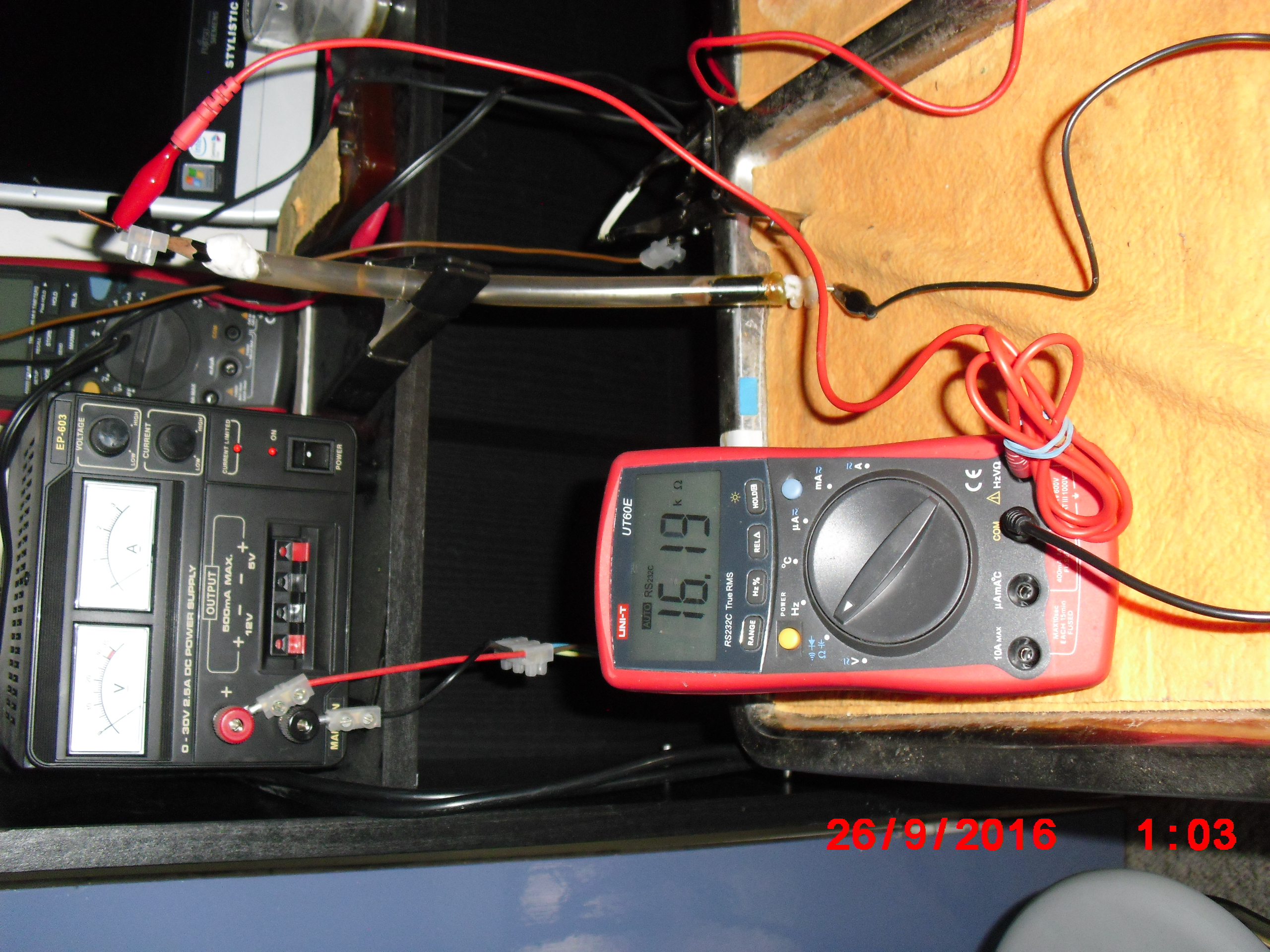
In Picture 28 you can see that the circuit resistance is 16.19 k Oms.

Picture 29

In Picture 29 you can see that the circuit resistance is 16.24 k Oms.

Picture 30

In Picture 30 you can see the restance through the graphite in the pencil stub is 029.9 Ohms

Picture 31

In Picture 31 you can see the resistance through the graphite in the pencil stub is 029.9 Ohms and this confirms that this measurement is repeatable and constant. This is one of the pencil stubs that is used to connect the salt water through the electrical connector and copper to the instrument.

Picture 32

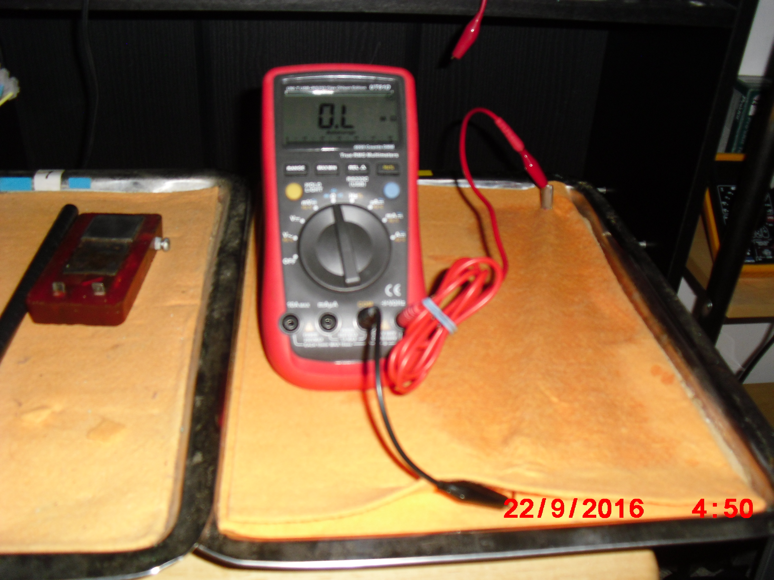
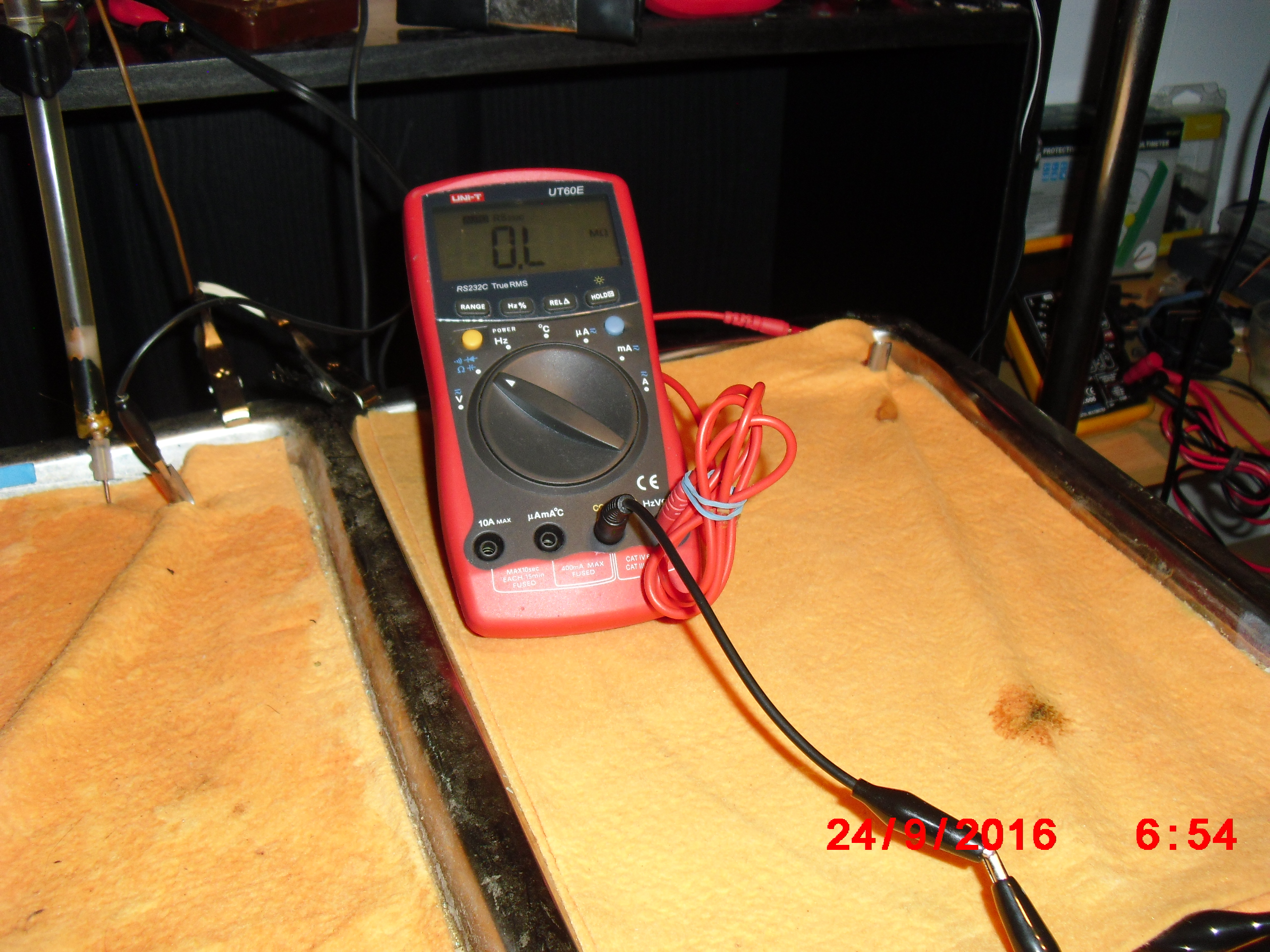
You will see that the meter is set to measure Ohms and reads O.L which means OverLoad M Ohms. The common is connected to the pencil stub graphite in the empty pipe and the other pole of the meter is connected to the raised metal tab on the pipe metal itself.

Picture 33

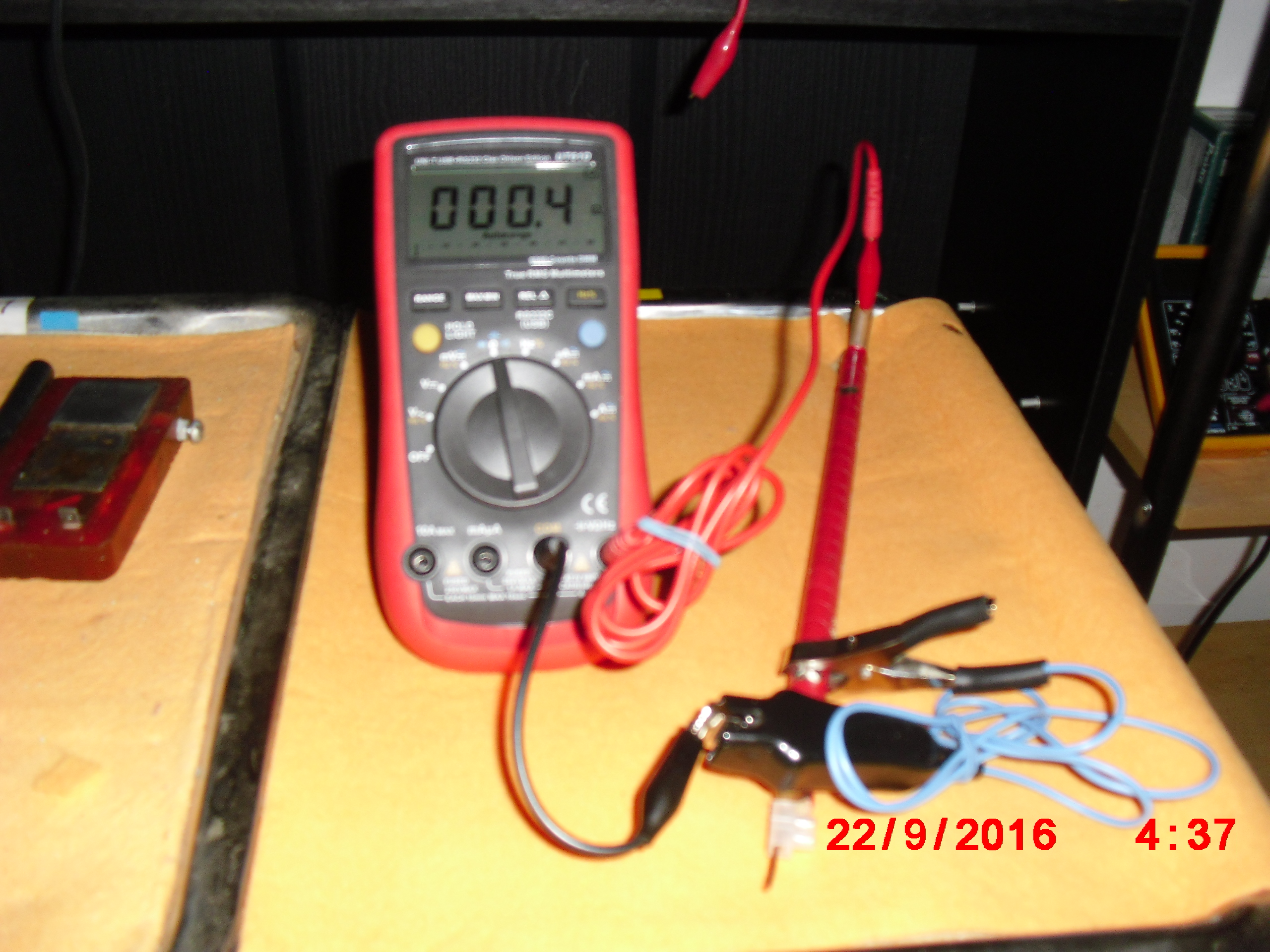
In Picture 32 you will see that the common pole of the meter is connected to a croc clip that is clamped over the near coating fault of the pipe and the resulting measurement is 000.4 Ohms

Picture 34

Picture 33 shows the measurement between the graphite in the empty pipe and the raised metal tab of the pipe. It is still O.L M Ohms

Picture 35

I have now wetted the cloth covering the pipe and it is in contact with the two coating faults on the top of the pipe.

Picture 36

Picture 35 shows 29.36 k Ohm resistance in the circuit from the common that is connected to the cloth through the two coating faults to the pipe metal and through the red lead to the meter.

Picture 37

Picture 37 shows the resistance has risen to 35.43 k Ohms two minutes later, so I have a glass of tap water ready to measure the effect of soaking the cloth.

Picture 38

Picture 38 shows 25.22 k Ohms due to the soaking of the cloth. This is the same as experienced during CIPS and DCVG surveys when measurement are taken over very dry ground.

Picture 39

Picture 39 was taken a minute after Picture 38 and shows that the measuring circuit resistance has increased to 26.81 k Ohms as the water soaks away from point of contact between the croc clip and the cloth.

Picture 40

Picture 40 is a repeat of a previous measurement to prove that the data is repeatedly observable as required by the scientific method.

Picture 41

Picture 41 shows the measuring circuit resistance to be 35.46 when the common is connected to the cloth and the other input pole is connected to the pipe metal. The lemon juice is ready to pour onto the location of the nearest coating fault.

Picture 42

Picture 42 shows the measuring circuit resistance to be 32.65 when the common is connected to the cloth and the other input pole is connected to the pipe metal. The lemon juice has been poured onto the location of the nearest coating fault.



Picture 43

Picture 43 shows the measuring circuit resistance to be 32.66 when the common is connected to the cloth and the other input pole is connected to the pipe metal. This picture was taken five minutes after the lemon juice has been poured onto the location of the nearest coating fault.

---

Equivalent pipe to soil measurements.

Picture 44

Picture 44 is the first of a series of equivalent 'pipe-to-soil potential' measurements that show that this is a voltage measurement between two variable potentials and that the copper/copper-sulphate electrode cannot be used as a reference potential in the way advocated by NACE and ICorr. The meter is displaying 560.7 mv with the probe positioned in the damp cloth beside the pipe and the common of the meter connected to the pipe metal.

Picture 45

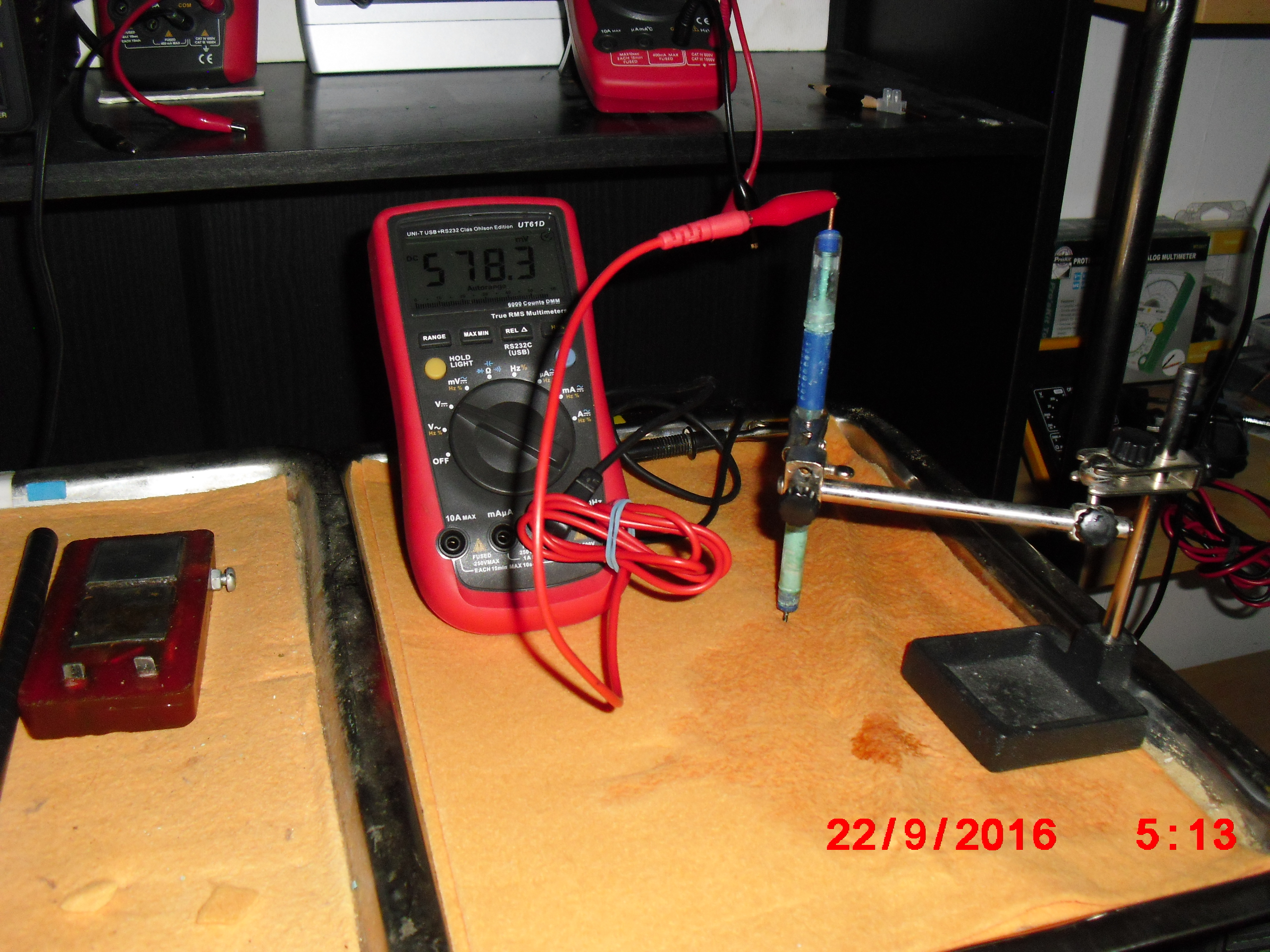
In Picture 45 you can see the measurement 578.3 mv and that the wiring has not been changed, only the position of the probe. This picture alone proves that we cannot use a copper/copper-sulphate electrode, as advised by NACE and ICorr, as a reference potential in equations that require the value of E denoting the potential energy at a node.

Picture 46

In Picture 46 you can see the measurement 593.9 mv and that the wiring has not been changed, only the position of the probe. This picture confirms that we cannot use a copper/copper-sulphate electrode, as advised by NACE and ICorr.

47

In Picture 47 you can see the measurement 589.5 mv and that the wiring has not been changed, only the position of the probe. This picture confirms that we cannot use a copper/copper-sulphate electrode, as advised by NACE and ICorr.

Picture 48

In Picture 48 you can see the measurement 0.628 volts and that the wiring has not been changed, only the position of the probe. The probe is exactly overthe far coating fault and subject to the EMF of the corrosion reaction at this location. This picture again confirms that we cannot use a copper/copper-sulphate electrode, as advised by NACE and ICorr.

Picture 49

In picture 49 you can see that the measurement 562.6 mv isdue to the position of the probe being exactly over the nearest coating fault. This picture again confirms that we cannot use a copper/copper-sulphate electrode, as advised by NACE and ICorr.

Picture 50

Picture 50 gives a clear view of the measurement 573.3and the position ofthe probe and wiring of the measuring circuit. This picture again confirms that we cannot use a copper/copper-sulphate electrode, as advised by NACE and ICorr.

Picture 51

In Picture 51 you can see the measurement 0.628 volts and that the wiring has not been changed, only the position of the probe. The probe is exactly over the far coating fault and subject to the EMF of the corrosion reaction at this location. This picture proves that it is possible to make repeated abservations as required by the scientific method. This picture again confirms that we cannot use a copper/copper-sulphate electrode, as advised by NACE and ICorr.

Picture 52

In Picture 52 you can see that the measurement 552.8 mv is due to the position of the probe being over the nearest coating fault.

---

The Alexander Cell

Picture 53

Picture 53 shows the resistance in the measuring circuit of the Alexander Cell when the top electrodes are NOT covered by a sample of the electrolyte.

Picture 54

Picture 54 shows the resistance in the Alexander Cell measuring circuit to be 040.7 k Ohm when the top electrodes are connected by the sample of the electrolyte.

Picture 55

Picture 55 shows that the circuit resistance in the Alexander Cell is reduced to 19.43 k Ohms when the electrolyte sample and the electrolyte on which the Alexander Cell stands have been soaked with more tap water.

Picture 56

Picture 56 shows that the circuit resistance in the Alexander Cell increases to 33.71 k Ohms as the electrolyte sample and the electrolyte on which the Alexander Cell stands dries out a minute later.

Picture 57

Picture 57 shows 32.83 k Ohms from a different angle so that you can see the circuit more clearly.

---

The black coated pipe

Picture 58

Picture 58 Shows the Alexander Cell and the electrolyte sample, the black coated control pipe with two coating faults, the test graphite conducting link to the internal liquid, the plastic tube used to test thr principle of the measuremnt technique and the 'buried' red coated test pipe with the stains caused by the corrosion products after a day in situe.

Picture 59

Picture 59 shows the black coated pipe has been 'buried' with dry cloth.

Picture 60

Picture 60 shows the red coated pipe exposed to show the corrosion products on the underside of the covering cloth and the graphite connection at the near end.

Picture 61

Picture 61 shows the reading of 1.1 Ohms between the close end of the black coatedpipe and the far end raised metal tab, with the covering cloth wet to connect the two coating faults.

Picture 62

Picture 62 shows the same circuit after 1 minute when the cloth has drained drier thus making more resistance in the external path of the 9 volt driven current.

---

Resistance of salt water in plastic tube.



Picture 63

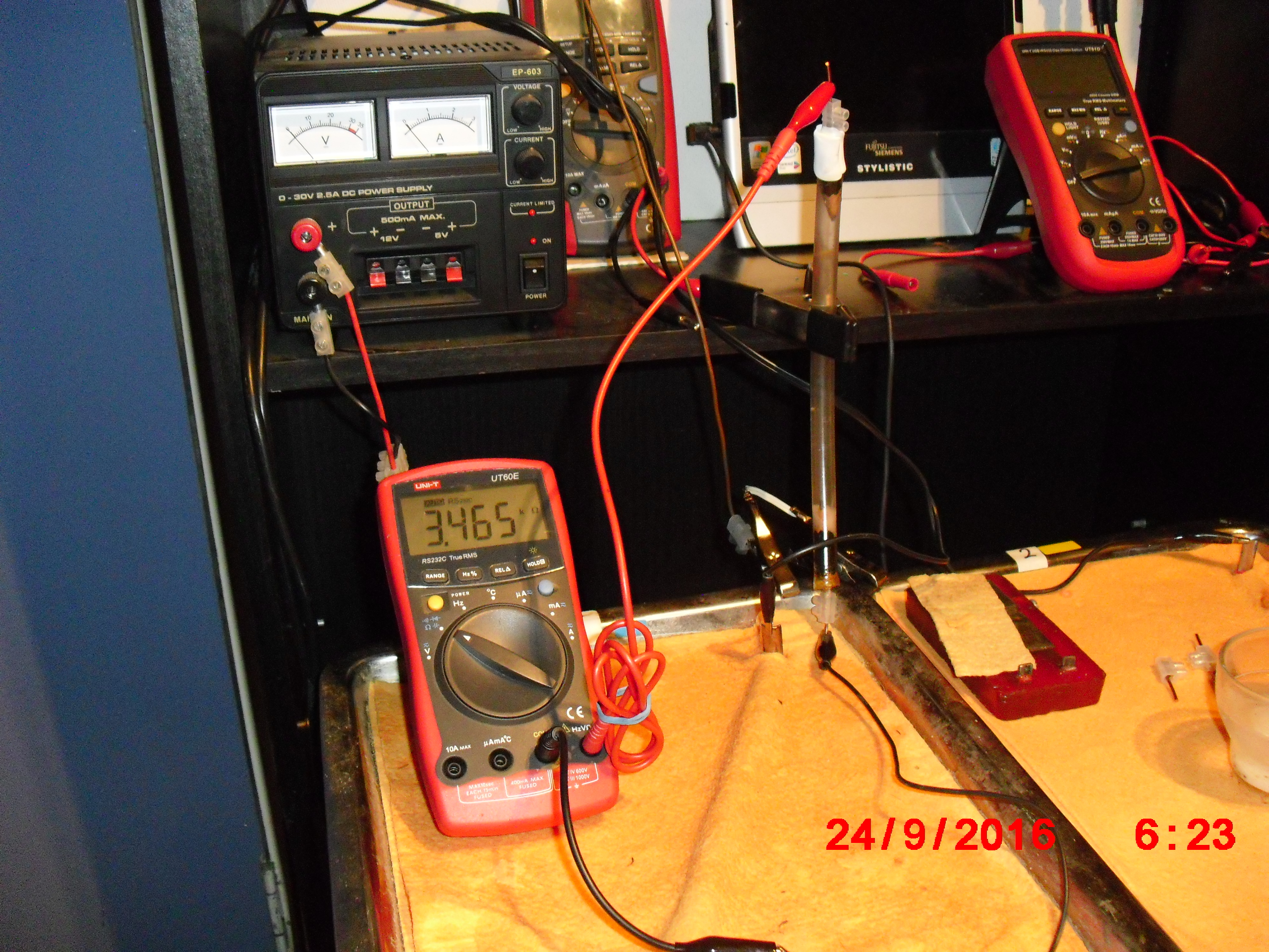
Picture 63 shows the resistance of the salt water in the plastic tube to be 3.465 k Ohms

Picture 64

Picture 64 shows the resistance of the salt water in the plastic tube to be 07.02 k Ohms

Picture 65

Picture 65 shows the resistance of the salt water in the plastic tube to be 04.31 k Ohms when the tube is lying down. In this picture you can see the measuring circuit and reading more clearly.

Picture 66

Picture 66 shows the resistance of the salt water in the plastic tube to be 2.603 k Ohms when the tube is lying down.

Picture 67

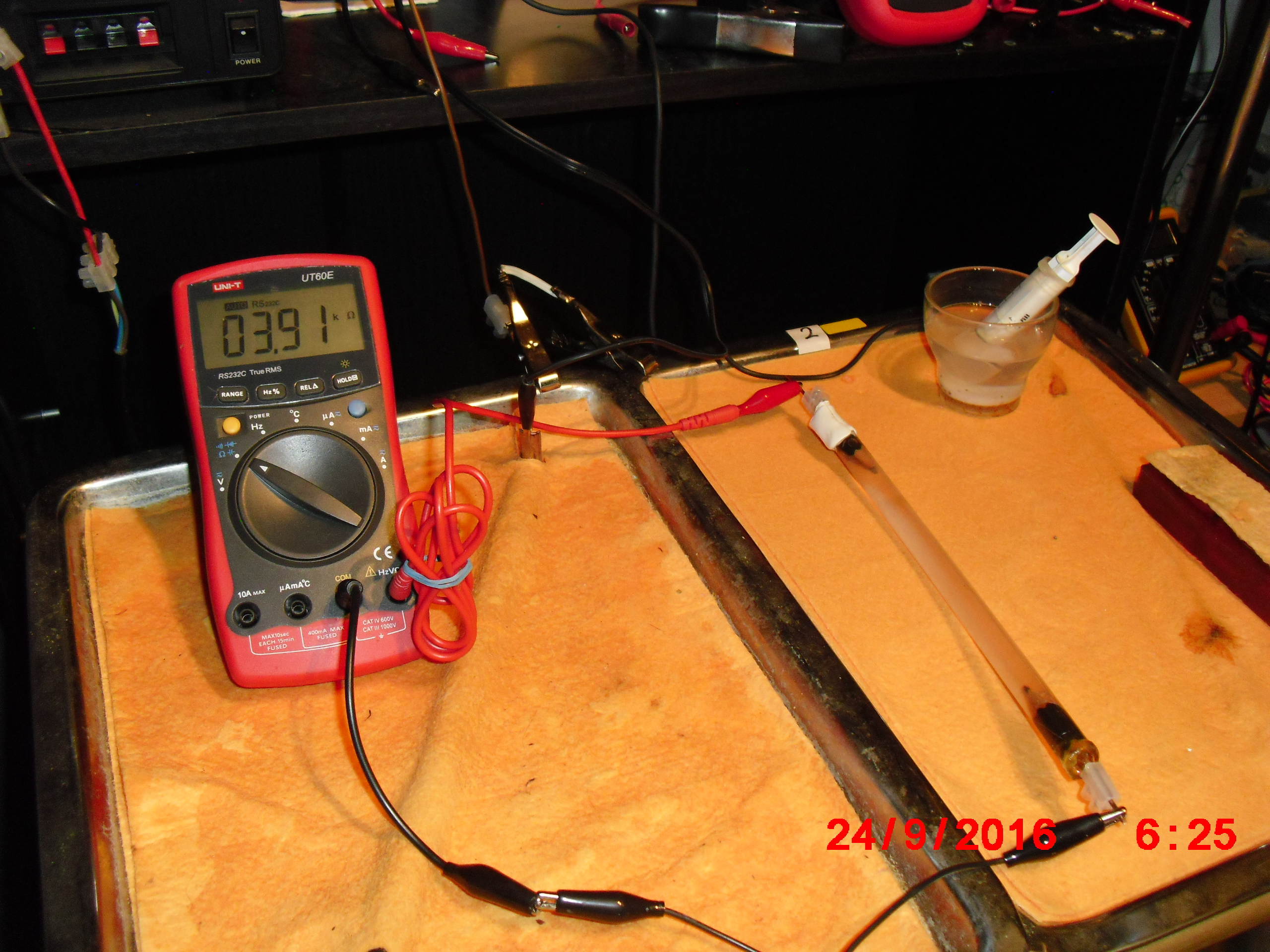
Picture 67 shows the resistance of the salt water in the plastic tube to be 03.91 k Ohms when the tube is lying down.

---

Picture 68
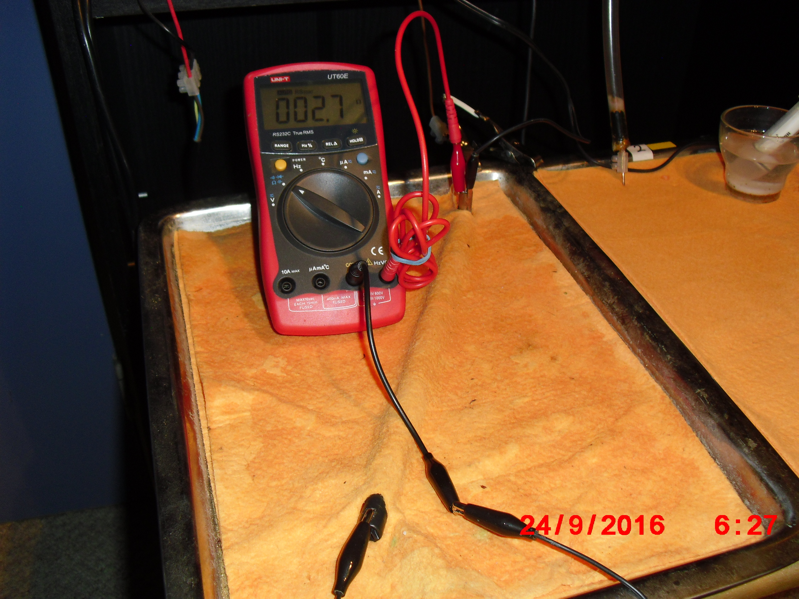
Picture 68 is another resistance measurement of the metal of the black coated pipewhen covered with the damp cloth. 002.7 Ohms



Picture 69

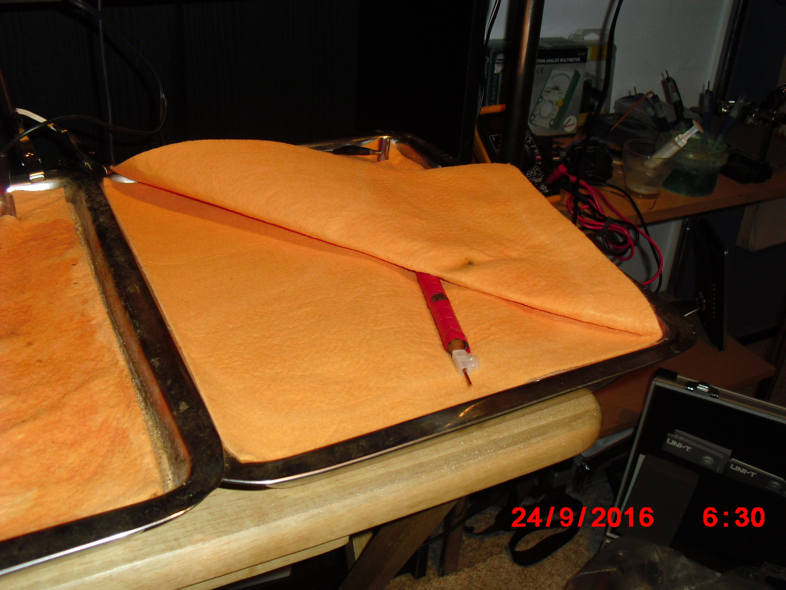
Picture 69 Shows the red coated pipe partly uncovered with the corrosion product from the close coating fault clearly visible.



Picture 70

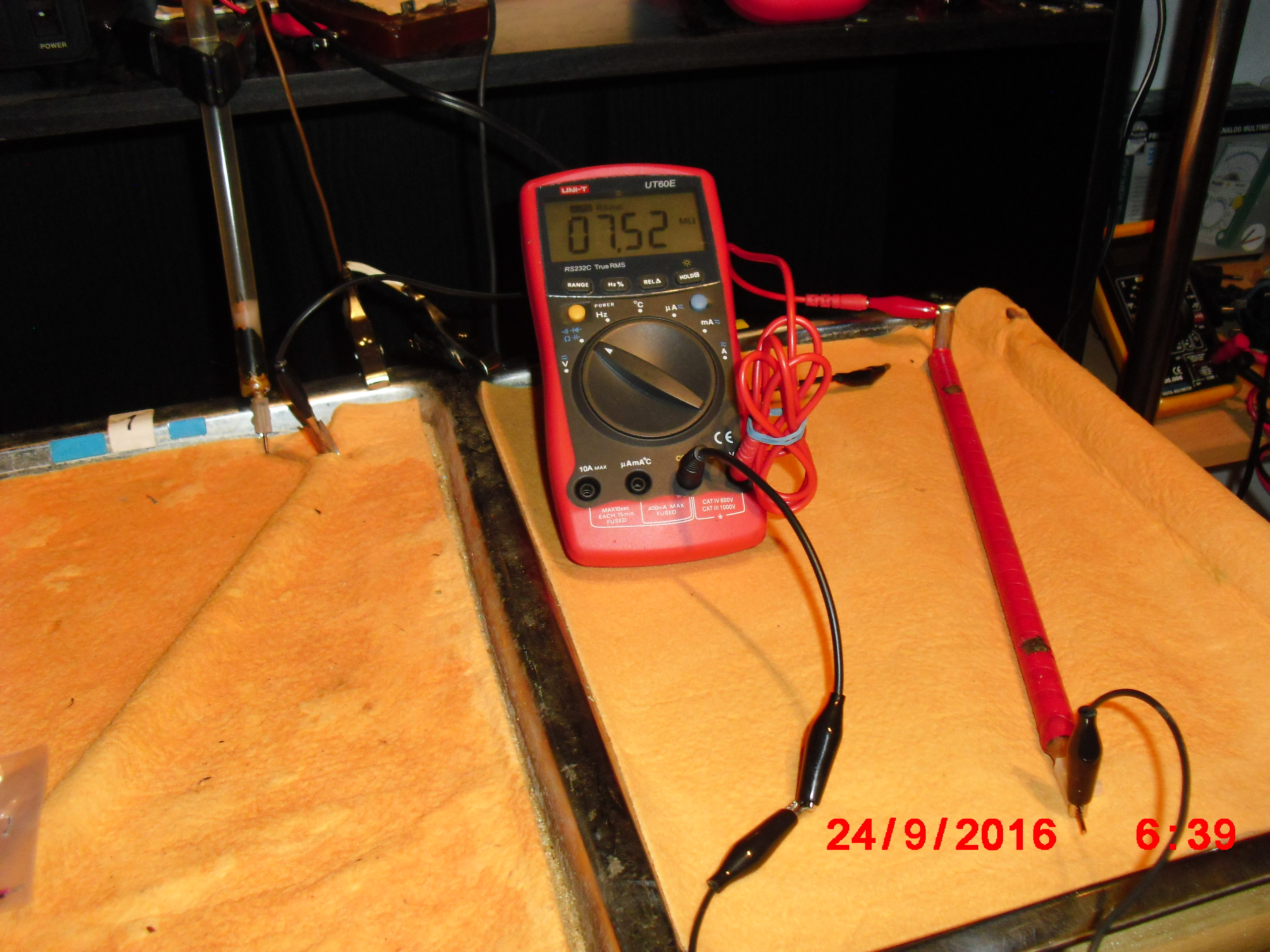
Picture 70 shows circuit resistance of 07.52 Mega Ohms through the graphite, the salt water to the metal tab of the pipe

Picture 71

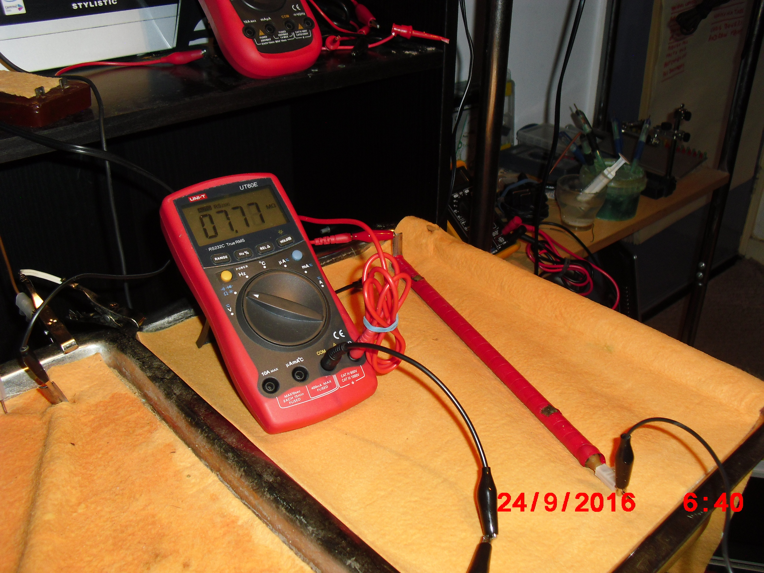
Picture 71 shows circuit resistance of 07.77 Mega Ohms one minute later through the same circuit viewed from a different angle.

Picture 72

Picture 72 shows circuit resistance of 1.589 Mega Ohms 8 minutes later through graphite, salt water, graphite circuit.

Picture 73

Picture 73 shows circuit resistance of 1.573 Mega Ohms through graphite, salt water, graphite circuit.

Picture 74

Picture 74 shows circuit resistance of 1.688 Mega Ohms through graphite, salt water, graphite circuit.

Picture 75

Picture 75 shows circuit resistance of 17.25 Mega Ohms through graphite, salt water, graphite circuit with the damp cloth covering.

Picture 76

Picture 76 shows circuit resistance of 17.82 Mega Ohms through graphite, salt water, graphite circuit with the damp cloth covering.

Picture 77

Picture 77 shows circuit resistance of 22.21 Mega Ohms through graphite, salt water, graphite circuit with the damp cloth covering.

Picture 78

Picture 78 shows that there is O.L Mega Ohms through the cicuit from the common pole through the cloth to cating faults to the metal through the salt water to the graphite to the meter.

Picture 79

Picture 79 shows 19.92 k Ohms from the damp cloth through the coating faults to the raised metal tab.

Picture 80

Picture 80 shows 23.48 k Ohms from the damp cloth through the coating faults to the raised metal tab.

Picture 81

Picture 81 shows O.L M Ohms between the graphite salt water inside the pipe and the graphite.

Picture 82

Picture 82 shows O.L M Ohms between the graphite salt water inside the pipe and the graphite.

Picture 83

Picture 83 shows O.L M Ohms between the graphite salt water inside the pipe and the graphite.

Picture 84

Picture 84 shows O.L M Ohms (on the left hand meter) between the graphite to the salt water inside the pipe and to the graphite at the other end. The meter on the right shows 4.689 k Ohms between the wet cloth, through the coating faults to the raised metal tab. In this way we can compare the two circuit resistances. Each of these meters utilises a 9 volt battery and Ohms law to display the results. R=V/I

Picture 85

Picture 85 shows that I have now connected the meter on the left to read the resistance in the metal of the black coated pipe and that is too low to be measured on this meter. I have stood the red coated pipe against the shelf above the tray and connected the right hand meter to the graphite - salt water - graphite circuit. This shows the salt water circuit as having 385.6 Mega Ohms resistance. When it was lying down it was off scale of the meter so standing it up has somehow reduced the resistance of this particular circuit.

Picture 86

Picture 86 was taken a minute later and shows the same connections with the red coated pipe standing up. The meter now shows 405.9 Mega Ohms. We need an explanation for this increase in resistance.

Picture 87

Picture 87 was taken a minute later and shows the same connections with the red coated pipe standing up. The meter now shows 421.7 Mega Ohms. The resistance has again increased.



Picture 88

Picture 88 shows that I have laid the red pipe down on top of the cloth in the right hand tray and the resistaance through the salt water is now 300.9 k Ohms This is a massive reduction of the resistance that needs explanation.

Picture 89

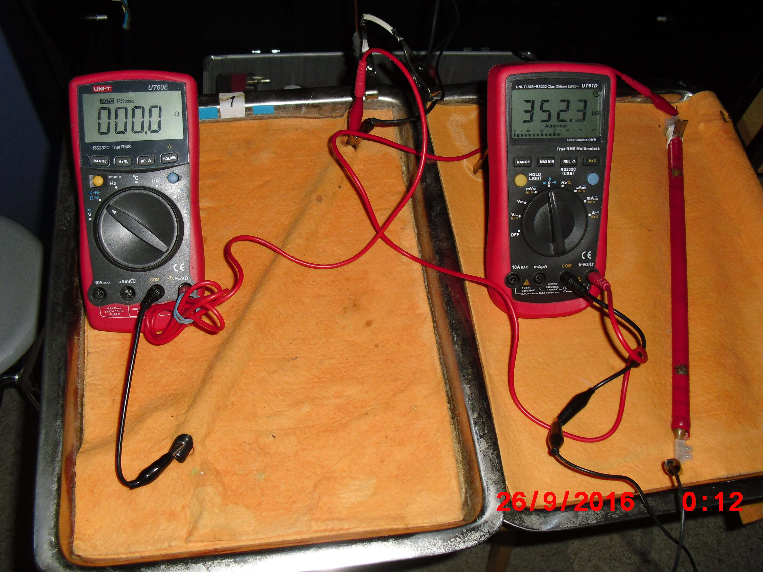
Picture 89 was taken a minute later and shows a resistance of 352.3 k Ohms through the salt water.

Picture 90

Picture 90 was taken a minute later and shows a resistance of 376.5 k Ohms through the salt water.

Picture 91

---

The impressed current cathodic protection system

Picture 92



Picture 93



Picture 94



Picture 95



Picture 97



Picture 98



Picture 99



Picture 100